Examples

Examples to illustrate the use of ComputationGraphs.

Adam's method for optimization

Adam's gradient-based optimization can be easily implement using the recipe adam! which includes all the "messy" formulas. In this example, we use Adam's method to minimize a quadratic criterion of the form

\[ J(x) = \| A\, x -b \|^2\]

with respect to $x$. To construct of the computation graph that accomplishes this, we use:

using ComputationGraphs
graph = ComputationGraph(Float64)
A = variable(graph, 400, 300)
x = variable(graph, 300)
b = variable(graph, 400)
loss = @add graph norm2(times(A, x) - b)
theta = (;x,)
(;  eta, beta1, beta2, epsilon,
    init_state, state, next_state,
    next_theta, gradients) = adam!(graph; loss, theta)
end # hide

With this graph in place, the actual optimization can be carried out as follows:

Initialize Adam's parameters

set!(graph, eta, 2e-2)
set!(graph, beta1, 0.9)
set!(graph, beta2, 0.999)
set!(graph, epsilon, 1e-8)
end # hide

Initialize the problem data (randomly, but freezing the random seed for repeatability)

using Random
Random.seed!(0)
set!(graph, A, randn(size(A)))
set!(graph, b, randn(size(b)))
end # hide

Initialize the parameters to optimize (again randomly, but freezing the random seed for repeatability)

Random.seed!(0)
init_x=randn(Float64,size(x))
set!(graph, x, init_x)
end # hide

Initialize Adam's internal state

copyto!(graph, state, init_state)

Run Adam's iterations:

using BenchmarkTools, Plots
lossValue=get(graph,loss)
println("initial loss: ", lossValue)
states=(;state...,theta...)
next_states=(;next_state...,next_theta...)
nIterations=1000
losses=Vector{Float64}(undef,nIterations)
bmk = @benchmark for i in 1:$nIterations
    compute!($graph, $next_states)
    copyto!($graph, $states, $next_states)
    $lossValue=get($graph, $loss)
    $losses[i]=$lossValue[1]
end  setup =( # reinitialize x and solver for each new sample
        set!($graph, $x, $init_x), copyto!($graph, $state, $init_state)
    ) evals=1 # a single evaluation per sample
println("final loss: ", lossValue)
plt=Plots.plot(losses,yaxis=:log,ylabel="loss",xlabel="iteration",label="",size=(750,400))
end # hide

initial loss: fill(125008.67163886719)
final loss: fill(116.63722408535794)
GKS: cannot open display - headless operation mode active
BenchmarkTools.Trial: 91 samples with 1 evaluation per sample.
 Range (min … max):  32.845 ms …  36.920 ms  ┊ GC (min … max): 0.00% … 0.00%
 Time  (median):     33.062 ms               ┊ GC (median):    0.00%
 Time  (mean ± σ):   33.147 ms ± 465.079 μs  ┊ GC (mean ± σ):  0.00% ± 0.00%

     ▆▆▃█▇▂▁                                                   
  ▃▇████████▇▄▃▄▁▃▆▁▁▁▁▁▁▁▁▃▁▃▁▁▁▁▁▁▁▁▁▁▁▁▁▁▁▁▁▁▁▁▁▁▁▁▁▁▁▁▁▁▁▃ ▁
  32.8 ms         Histogram: frequency by time         34.8 ms <

 Memory estimate: 0 bytes, allocs estimate: 0.

As expected for a convex optimization, convergence is pretty smooth:

convergence plot

Note

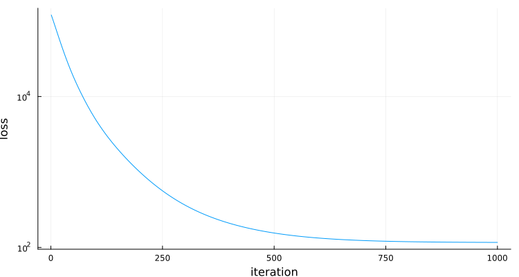
For @benchmark to reflect the time an actual optimization, we reset the optimization variable x and the solver's state at the start of each sample (using @benchmark's setup code).

Adam's method with projection

Suppose now that we wanted to add a "projection" to Adam's method to keep all entries of x positive. This could be done by simply modifying the next_theta produced by Adam to force all the entries of next_step.x to be positive, using the relu function:

next_theta = (x=relu(graph,next_theta.x),)

We can now repeat the previous steps (reinitializing everything for a fresh start):

set!(graph, x, init_x)
copyto!(graph, state, init_state)
lossValue=get(graph,loss)
println("initial loss: ", lossValue)
states=(;state...,theta...)
next_states=(;next_state...,next_theta...)
nIterations=1000
losses=Vector{Float64}(undef,nIterations)
bmk = @benchmark for i in 1:$nIterations
    compute!($graph, $next_states)
    copyto!($graph, $states, $next_states)
    $lossValue=get($graph,$loss)
    $losses[i]=$lossValue[1]
end  setup =( # reinitialize x and solver for each new sample
        set!($graph, $x, $init_x), copyto!($graph, $state, $init_state)
    ) evals=1 # a single evaluation per sample
println("final loss: ", lossValue)
plt=Plots.plot(losses,yaxis=:log,ylabel="loss",xlabel="iteration",label="",size=(750,400))
end # hide

initial loss: fill(125008.67163886719)
final loss: fill(249.7135504173925)
BenchmarkTools.Trial: 90 samples with 1 evaluation per sample.
 Range (min … max):  33.178 ms …  37.604 ms  ┊ GC (min … max): 0.00% … 0.00%
 Time  (median):     33.393 ms               ┊ GC (median):    0.00%
 Time  (mean ± σ):   33.431 ms ± 457.988 μs  ┊ GC (mean ± σ):  0.00% ± 0.00%

             ▅  ▅      ▂▂ ▅█▂ █  ▂▅  ▅                         
  ▅▁███▅█▅█▁██████▅▅▅████████▅██▅██▁▅██▁▁▅▅█▅▅▅▁▁▁▅▁▁▁▁▅▁▁▁▁▁▅ ▁
  33.2 ms         Histogram: frequency by time         33.7 ms <

 Memory estimate: 0 bytes, allocs estimate: 0.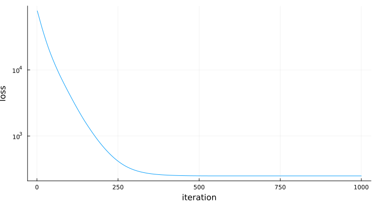

convergence plot

Note

For @benchmark to reflect the time an actual optimization, we reset the optimization variable x and the solver's state at the start of each sample (using @benchmark's setup code).

Neural network training

In this example, we combine the two recipes denseChain! and adam! to train and query a dense forward neural network of form:

    x[1]   = input
    x[2]   = activation(W[1] * x[1] + b[1])
    ...
    x[N-1] = activation(W[N-2] * x[N-2] + b[N-2])
    output = W[N-1] * x[N-1] + b[N-1]               # no activation in the last layer
    loss = some_loss_function(output-reference)

As in Neural-network recipes, our goal is to train a neural network whose input is an angle in the [0,2*pi] range with two outputs that return the sine and cosine of the angle. To accomplish this will use a network with 1 input, 2 output, a few hidden layers, and relu activation functions.

We start by using denseChain! to construct a graph that performs all the computations needed to do inference and compute the (training) loss function for the network. The computation graph will support:
- inference, i.e., compute the output for a given input;
- training, i.e., minimize the loss for a given set of inputs and desired outputs.
For training we will use a large batch size, but for inference we will only provide one input at a time.

using ComputationGraphs, Random
begin # end
graph=ComputationGraph(Float32)
hiddenLayers=[30,20,30]
nNodes=[1,hiddenLayers...,2]
(; inference, training, theta)=denseChain!(graph;
        nNodes,
        inferenceBatchSize=1,
        trainingBatchSize=5_000,
        activation=ComputationGraphs.relu,
        loss=:mse)
println("graph with ", length(graph), " nodes and ",ComputationGraphs.memory(graph)," bytes")

graph with 30 nodes and 3367440 bytes

where

nNodes is a vector with the number of nodes in each layer, starting from the input and ending at the output layer.
inferenceBatchSize is the number of inputs for each inference batch.
trainingBatchSize is the number of inputs for each training batch.
activation: is the activation function.
loss defines the loss to be the mean square error.

and the returned tuple includes

inference::NamedTuple: named tuple with the inference nodes: + input NN input for inference + output NN output for inference
training::NamedTuple: named tuple with the training nodes: + input NN input for training + output NN output for training + reference NN desired output for training + loss NN loss for training
theta::NamedTuple: named tuple with the NN parameters (all the matrices W and b)

We then use the adam! recipe add to the graph the computation needed to optimize the weights.

(;  eta, beta1, beta2, epsilon,
    init_state, state, next_state,
    next_theta, gradients) = adam!(graph; loss=training.loss, theta=theta)
println("graph with ", length(graph), " nodes and ",ComputationGraphs.memory(graph)," bytes")

graph with 195 nodes and 8327772 bytes

where we passed to adam! the nodes that correspond to the neural network loss and use the neural network parameters as the optimization variables.

In return, we get back the nodes with Adam's parameters as well as the nodes needed for the algorithm's update.

We initialize the network weights with random (but repeatable) values. We use a function for this, to be able to call it many times.

function init_weights(graph,theta)
    Random.seed!(0)
    for k in eachindex(theta)
        set!(graph,theta[k],0.2*randn(Float32,size(theta[k])))
    end
end

We are almost ready to use Adam's iterative algorithm, similarly to what was done in Adam's method for optimization. However, and as commonly done in training neural networks, we will use a different random set of training data at each iteration.
To this effect, we create a "data-loader" function that will create a new set of data at each iteration:

function dataLoader!(input,output)
    for k in eachindex(input)
        input[k]=(2*pi)*rand(Float32)
        output[1,k]=sin(input[k])
        output[2,k]=cos(input[k])
    end
end

Now we are indeed ready for training:

using BenchmarkTools, Plots
# Initialize Adam's parameters
set!(graph, eta, 8e-4)
set!(graph, beta1, 0.9)
set!(graph, beta2, 0.999)
set!(graph, epsilon, 1e-8)
# create arrays for batch data
input=Array{Float32}(undef,size(training.input))
output=Array{Float32}(undef,size(training.reference))
# Create array to save losses
nIterations=1_000
losses=Vector{Float32}(undef,nIterations)
# Adam iteration
states=(;state...,theta...)
next_states=(;next_state...,next_theta...)
bmk = BenchmarkTools.@benchmark begin
    copyto!($graph, $state, $init_state)     # initialize optimizer
    for i in 1:$nIterations
        dataLoader!($input,$output)          # load new dataset
        set!($graph,$training.input,$input)
        set!($graph,$training.reference,$output)
        compute!($graph, $next_states)          # compute next optimizer's state
        copyto!($graph, $states, $next_states)     # update optimizer's state
        lossValue=get($graph, $training.loss)
        $losses[i]=lossValue[1]
    end
end setup=(init_weights($graph,$theta)) evals=1 # a single evaluation per sample
println("final loss: ", get(graph,training.loss))
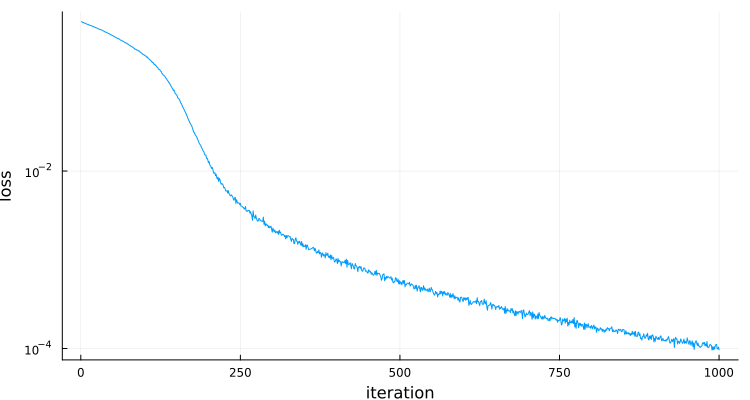
plt=Plots.plot(losses,yaxis=:log,
    ylabel="loss",xlabel="iteration",label="",size=(750,400))

final loss: fill(9.6966294f-5)
BenchmarkTools.Trial: 5 samples with 1 evaluation per sample.
 Range (min … max):  3.548 s …  3.572 s  ┊ GC (min … max): 0.00% … 0.00%
 Time  (median):     3.556 s             ┊ GC (median):    0.00%
 Time  (mean ± σ):   3.559 s ± 9.652 ms  ┊ GC (mean ± σ):  0.00% ± 0.00%

  █            █     █                     █             █ 
  █▁▁▁▁▁▁▁▁▁▁▁▁█▁▁▁▁▁█▁▁▁▁▁▁▁▁▁▁▁▁▁▁▁▁▁▁▁▁▁█▁▁▁▁▁▁▁▁▁▁▁▁▁█ ▁
  3.55 s        Histogram: frequency by time        3.57 s <

 Memory estimate: 0 bytes, allocs estimate: 0.

In spite of not being a convex optimization, convergence is still pretty good (after carefully choosing the step size eta).

convergence plot

We can now check how the neural network is doing at computing the sine and cosine:

angles=0:.01:2*pi
outputs=Array{Float32}(undef,2,length(angles))
for (k,angle) in enumerate(angles)
    set!(graph,inference.input,[angle])
    (outputs[1,k],outputs[2,k])=get(graph,inference.output)
end
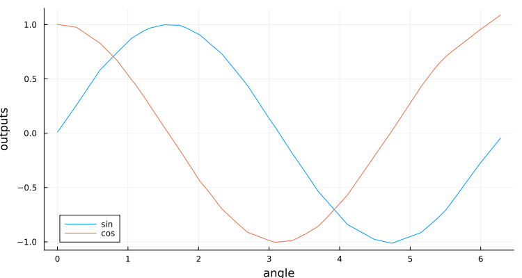
plt=Plots.plot(angles,outputs',
    xlabel="angle",ylabel="outputs",label=["sin" "cos"],size=(750,400))
end # hide

and it looks like the network is doing quite well at computing the sine and cosine:

inference

Warning

The code above does inference one angle at a time, which is quite inefficient. This could be avoided, by setting inferenceBatchSize to a value larger than 1.

Doing it with Flux

The same problem can be solved with Flux.jl:

We start by building a similar network and an Adam's optimizer

using Flux
model=Chain(
    [Dense(
        Matrix{Float32}(undef,nNodes[k+1],nNodes[k]),
        Vector{Float32}(undef,nNodes[k+1]),Flux.relu)
    for k in 1:length(nNodes)-2]...,
    Dense(
        Matrix{Float32}(undef,nNodes[end],nNodes[end-1]),
        Vector{Float32}(undef,nNodes[end]),identity)
)
optimizer=Flux.Adam(8e-4,(0.9,0.999),1e-8)

We initialize the network weights with random (but repeatable) values. We use a function for this, to be able to call it many times.

function init_weights(model)
    Random.seed!(0)
    for k in eachindex(model.layers)
        model.layers[k].weight .= 0.2*randn(Float32,size(model.layers[k].weight))
        model.layers[k].bias .= 0.2*randn(Float32,size(model.layers[k].bias))
    end
end

We now train the network

# create arrays for batch data
input=Array{Float32}(undef,size(training.input))
output=Array{Float32}(undef,size(training.reference))
# Create array to save losses
nIterations=1_000
losses=Vector{Float32}(undef,nIterations)
bmk = BenchmarkTools.@benchmark begin
    opt_state=Flux.setup($optimizer,$model)      # initialize optimizer
    for i in 1:$nIterations
        dataLoader!($input,$output)              # load new dataset
        loss,grad = Flux.withgradient(           # compute loss & gradient
            (m) -> Flux.mse(m($input),$output),
            $model)
        Flux.update!(opt_state,$model,grad[1])   # update optimizer's state
        $losses[i]=loss
    end
end setup=(init_weights($model)) evals=1 # a single evaluation per sample
println("final loss: ", get(graph,training.loss))
plt=Plots.plot(losses,yaxis=:log,
    ylabel="loss",xlabel="iteration",label="",size=(750,400))

final loss: fill(9.6966294f-5)
BenchmarkTools.Trial: 5 samples with 1 evaluation per sample.
 Range (min … max):  3.001 s …   3.053 s  ┊ GC (min … max): 5.97% … 5.85%
 Time  (median):     3.016 s              ┊ GC (median):    5.89%
 Time  (mean ± σ):   3.023 s ± 22.614 ms  ┊ GC (mean ± σ):  5.76% ± 0.29%

  █ █             █                        █              █ 
  █▁█▁▁▁▁▁▁▁▁▁▁▁▁▁█▁▁▁▁▁▁▁▁▁▁▁▁▁▁▁▁▁▁▁▁▁▁▁▁█▁▁▁▁▁▁▁▁▁▁▁▁▁▁█ ▁
  3 s            Histogram: frequency by time        3.05 s <

 Memory estimate: 4.72 GiB, allocs estimate: 371101.

We can see similar convergence for the network, but Flux leads to a very large number of allocations, which eventually result in higher computation times.

Examples

Contents

Adam's method for optimization

Adam's method with projection

Neural network training

Doing it with Flux